How has New York City's tree population changed over time?
Created by
Eric J.S.
Posted
May 9, 2022
Last updated
May 9, 2022
Category
Analysis
Tools Used
RSQLPython
Summary
New York City keeps an incredible amount of data. Every 10 years they release a dataset cataloging all the street trees in the city. So, how has NYC’s tree population changed over time?
I wanted this project to emphasize data exploration rather than data analysis, so I used the question above as a guide rather than a target. My focus was to display interesting charts, statistics, and maps with R and SQL.
Data Acquisition and Preparation
I first found the dataset on Kaggle, but realized it was lacking good descriptions for the data fields. I managed to find the same datasets on NYC’s official data hub.
1995 Street Tree Census - NYC Open Data
It’s worth noting that this data is crowdsourced by volunteers and may not be entirely accurate. You can read more about New York City’s tree census here.
I used Python to convert the CSV files to an SQLite database. SQLite has the advantages of being self-contained and supported by Python, R, and ArcGIS Pro. Optionally, I could have read the CSV files into R and stored them in memory, but these datasets combine to over a gigabyte and I didn’t want that much data sitting in memory for such a simple analysis. In a professional setting, data would most likely be stored in a network database anyway.
# PYTHON
# Uses pandas to create a new SQLite DB from a list of files

import sqlite3
import pandas

# Options
# this database will be created or overwritten
# use the .sqlite extension for ArcGIS Pro compatibility
sqliteDB = r"C:\path\to\database.sqlite"
# list the files (tables) to be added to the database
fileList = [
    r"C:\path\to\dataInCsvFormat1.csv",
    r"C:\path\to\dataInCsvFormat2.csv",
    r"C:\path\to\dataInCsvFormat3.csv"
]

# read a CSV and return a pandas dataframe
def readCSV(csvFileName):
    print("read csv file: " + csvFileName)
    return pandas.read_csv(csvFileName)

if __name__ == '__main__':
    # open a connection to the database
    conn = sqlite3.connect(sqliteDB)
    # for each file in the file list above
    for file in fileList:
        # determine the file extension
        splitFile = file.split(".")
        fileExt = splitFile[-1]
        # get the name of the file
        # this will be used as the table name in the database
        name = splitFile[-2].split("\\")[-1]
        # if the file extension is csv, use the readCSV function
        # this allows the ability to parse other file types in the future
        if fileExt == "csv":
            df = readCSV(file)
        # print the first few table rows to preview the data being added
        print(df.head())
        # add the dataframe to the SQLite database
        df.to_sql(name=name, con=conn, if_exists="replace", chunksize=1000)
    # commit the changes to the database
    conn.commit()
    # close the database connection
    conn.close()
Analysis
My general process for this entire analysis was to extract the necessary data with SQL and display the data in a chart with R. I used ggplot2 and ggmap for my visualizations in R. They work well together and allow for extensive customization.
# R
# load libraries

# use tidyverse for utility (includes ggplot2)
library(tidyverse)
# use ggmap to plot maps
library(ggmap)
# use DBI for database connections
library(DBI)

# connect to sqlite database
treeCensus <- dbConnect(RSQLite::SQLite(), "C:/path/to/NycTreeCensus.sqlite")

# register a google maps API key for ggmap
register_google(key="jibberish")
Tree Population Over Time
Let's begin by comparing tree population over time.
-- SQL
-- get the number of rows in each table
SELECT count( * ) AS count
FROM new_york_tree_census_1995
UNION ALL
SELECT count( * ) AS count
FROM new_york_tree_census_2005_fixed
UNION ALL
SELECT count( * ) AS count
FROM new_york_tree_census_2015;
# R
# the SQL query above is stored in variable q as a string
# store the result from the query
treePop <- dbGetQuery(treeCensus, q)
# add years column to table
treePop$year <- c(1995, 2005, 2015)
# show the first few rows
head(treePop)
# count year
# 1 516989 1995
# 2 592372 2005
# 3 683788 2015
# plot the data
# verticalTheme is a theme I defined and is unnecessary to create this plot
# lineColor is defined in the theme
# you can find the theme definition at the bottom of this post
ggplot(data=treePop, aes(y=count, x=year)) +
geom_line(size=1,
color=lineColor) +
geom_point(shape=21,
size=3,
stroke=1.5,
fill="white",
color=lineColor) +
labs(title="Street Tree Population in NYC",
x="Year",
y="Number of Trees"
) +
verticalTheme +
scale_y_continuous(limits=c(0, 800000),
expand=c(0,0),
labels=scales::comma) +
scale_x_continuous(expand=c(0,0.5))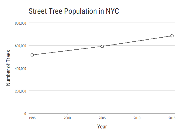
Alive Trees Over Time
Tree health is logged in each census, but the allowed values change each time. Instead, let’s display living trees as an area under our tree population line. This shows the living trees as a portion of the total trees, but also allows us to compare living trees over time.
-- SQL
-- get the alive trees from each table
-- each census has a different way of defining dead trees
SELECT count( * ) AS alive_count
FROM new_york_tree_census_1995
WHERE status != "Dead" AND
      status != "Planting Space" AND
      status != "Shaft" AND
      status != "Stump" AND
      status != "Unknown"
UNION ALL
SELECT count( * ) AS alive_count
FROM new_york_tree_census_2005_fixed
WHERE status != "Dead"
UNION ALL
SELECT count( * ) AS alive_count
FROM new_york_tree_census_2015
WHERE status != "Dead" AND
      status != "Stump";
# R
# the SQL query above is stored in variable q as a string
treesAlive <- dbGetQuery(treeCensus, q)
head(treesAlive)
# alive_count
# 1 471748
# 2 584252
# 3 652173
# add alive counts to tree table
treePop$alive_count <- treesAlive$alive_count
head(treePop)
# count year alive_count
# 1 516989 1995 471748
# 2 592372 2005 584252
# 3 683788 2015 652173
# create plot
# plot two areas, one for total trees and one for alive trees
ggplot(data=treePop, aes(x=year, y=count)) +
geom_area(aes(fill="Dead")) +
geom_area(aes(x=year, y=alive_count, fill="Alive")) +
geom_line(size=1,
color=lineColor) +
geom_point(shape=21,
size=3,
stroke=1.5,
fill="white",
color=lineColor) +
labs(title="Street Tree Population in NYC",
x="Year",
y="Number of Trees",
fill="Status"
) +
verticalTheme +
scale_y_continuous(limits=c(0, 800000),
expand=c(0,0),
labels=scales::comma) +
scale_x_continuous(expand=c(0,0.5)) +
scale_fill_manual(values=c("#8db39f", "#d4cbc0"))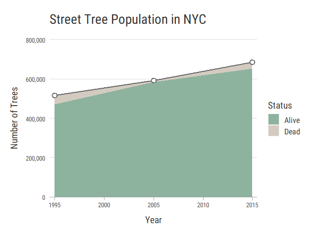
Top 10 Tree Genuses Over Time
Tree species are also recorded in each census, but the spellings don’t always match between years. I extracted the tree genuses, normalized by population, and compared those instead.
-- SQL
-- get the unique tree genuses and their counts
-- Sqlite doesn't support procedures, so it's a lot of repetition
SELECT *
FROM (
         SELECT *
         FROM (
                  SELECT CASE instr(trim(spc_latin), " ")
                            WHEN 0 THEN lower(trim(spc_latin) )
                            ELSE lower(substr(spc_latin, instr(trim(spc_latin), " "), -100) )
                            END genus,
                         count( * ) AS count,
                         ( (count( * ) * 1.0) / (
                                                    SELECT count( * )
                                                    FROM new_york_tree_census_2015
                                                )
                         ) * 100 AS pct,
                         "2015" AS year
                  FROM new_york_tree_census_2015
                  GROUP BY genus
              )
         UNION
         SELECT *
         FROM (
                  SELECT CASE instr(trim(spc_latin), " ")
                            WHEN 0 THEN lower(trim(spc_latin) )
                            ELSE lower(substr(spc_latin, instr(trim(spc_latin), " "), -100) )
                            END genus,
                         count( * ) AS count,
                         ( (count( * ) * 1.0) / (
                                                    SELECT count( * )
                                                    FROM new_york_tree_census_2005_fixed
                                                )
                         ) * 100 AS pct,
                         "2005" AS year
                  FROM new_york_tree_census_2005_fixed
                  GROUP BY genus
              )
         UNION
         SELECT *
         FROM (
                  SELECT CASE instr(trim(spc_latin), " ")
                            WHEN 0 THEN lower(trim(spc_latin) )
                            ELSE lower(substr(spc_latin, instr(trim(spc_latin), " "), -100) )
                            END genus,
                         count( * ) AS count,
                         ( (count( * ) * 1.0) / (
                                                    SELECT count( * )
                                                    FROM new_york_tree_census_1995
                                                )
                         ) * 100 AS pct,
                         "1995" AS year
                  FROM new_york_tree_census_1995
                  GROUP BY genus
              )
     )
     JOIN
     (
         SELECT *,
                count( * ) AS count_total
         FROM (
                  SELECT CASE instr(trim(spc_latin), " ")
                    WHEN 0 THEN lower(trim(spc_latin) )
                    ELSE lower(substr(spc_latin, instr(trim(spc_latin), " "), -100) )
                    END genus_total
                  FROM new_york_tree_census_1995
                  UNION ALL
                  SELECT CASE instr(trim(spc_latin), " ")
                    WHEN 0 THEN lower(trim(spc_latin) )
                    ELSE lower(substr(spc_latin, instr(trim(spc_latin), " "), -100) )
                    END genus_total
                  FROM new_york_tree_census_2005_fixed
                  UNION ALL
                  SELECT CASE instr(trim(spc_latin), " ")
                    WHEN 0 THEN lower(trim(spc_latin) )
                    ELSE lower(substr(spc_latin, instr(trim(spc_latin), " "), -100) )
                    END genus_total
                  FROM new_york_tree_census_2015
              )
         GROUP BY genus_total
     )
     ON genus = genus_total
ORDER BY count_total DESC,
         year;
# R
# the SQL query above is stored in variable q as a string
treeGenus <- dbGetQuery(treeCensus, q)
head(treeGenus)
# genus count pct year genus_total count_total
# 1 acer 173960 33.64868 1995 acer 399671
# 2 acer 136972 23.12263 2005 acer 399671
# 3 acer 88739 12.97756 2015 acer 399671
# 4 platanus 88055 17.03228 1995 platanus 264598
# 5 platanus 89529 15.11364 2005 platanus 264598
# 6 platanus 87014 12.72529 2015 platanus 264598
# remove NA value from table
treeGenus <- drop_na(treeGenus)
# subset the top 10 genus
# the table is already sorted by genus total count
# there are 3 rows per genus, so limit the table to the first 30 rows
tgTop <- head(treeGenus, n=30)
# bar plot of the common genus names
ggplot(data=tgTop) +
geom_col(mapping=aes(x=genus, y=pct, fill=year), position="dodge", width=0.7) +
scale_y_continuous(limits=c(0, 35), expand=c(0,0)) +
scale_x_discrete(labels=str_to_title) +
labs(title="NYC Street Tree Genus Population",
x="Tree Genus",
y="Percentage of Tree Population",
fill="Year"
) +
verticalTheme +
scale_fill_viridis_d(direction=-1)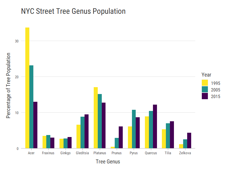
Mapping a Subset of Trees
The tree census provides a latitude, longitude, and address for each tree. Since there are over 600,000 trees in New York City, plotting them just creates a blob. Let’s zoom in to the neighborhood of Wallabout near Brooklyn and compare the maps from 1995 and 2015. Wallabout conveniently has the zip code 11205 which will make it easy to isolate trees to that area.
-- SQL
-- trees from Wallabout, NY in 1995
SELECT status, longitude, latitude
FROM new_york_tree_census_1995
WHERE zip_new = 11205;

-- trees from Wallabout, NY in 2015
SELECT status, longitude, latitude
FROM new_york_tree_census_2015
WHERE zipcode = 11205;
# R
# the SQL query above is stored in variable q as a string
treeSample <- dbGetQuery(treeCensus, q)
# drop empty values from the table
treeSample <- drop_na(treeSample)
head(treeSample)
# status longitude latitude
# 1 Alive -73.96905 40.69390
# 2 Alive -73.95652 40.69134
# 3 Stump -73.96766 40.69201
# 4 Alive -73.96869 40.68939
# 5 Alive -73.95163 40.68990
# 6 Alive -73.97234 40.69026
# get longitude and latitude values
lon <- treeSample$longitude
lat <- treeSample$latitude
# create a bounding box from the lat and lon values
treeBB <- make_bbox(lon, lat)
# calculate the center of the bounding box
# this will not work for every hemisphere due to the nature of latitude and longitude
(treeCenter <- c((treeBB['left'] + treeBB['right'])/2,
(treeBB['top'] + treeBB['bottom'])/2))
# use google maps because it allows larger scales
# request black and white roadmap with no labels
# overlay (darken) the base map with white to improve visibility of tree points
ggmap(get_googlemap(center=treeCenter,
maptype="roadmap",
zoom=15,
color="bw",
style="feature:all|element:labels|visibility:off"),
darken=c(0.6, "white")) +
geom_point(data=treeSample,
mapping=aes(x=longitude, y=latitude),
stroke=0,
alpha=0.5,
color="palegreen4") +
theme_void()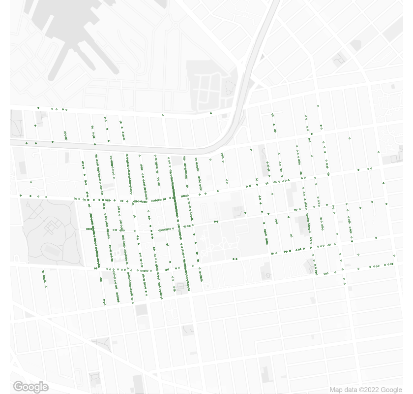 Street trees in Wallabout, NY 11205 in 1995.
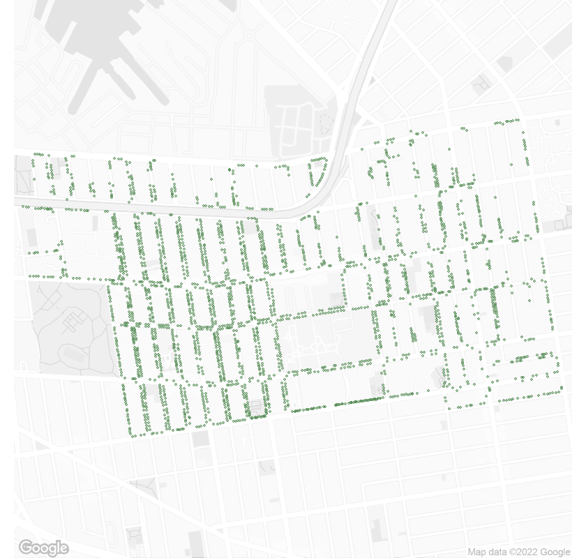 Street trees in Wallabout, NY 11205 in 2015.
Oldest Trees in the City
It would be interesting to see which street trees are the oldest in the city, but the ID for each tree corresponds to the planting spot and not the tree itself. We can make the assumption that if the tree is the same species in the same spot, it is the same tree. But, as previously discussed, the species are not always spelled the same between years, so we’ll match genuses instead.
To improve our accuracy, let’s add a third criteria where the tree diameter must be larger than a specific value. Tree diameters are recorded at approximately 4.5 feet above the ground, so they should provide some indication of tree age.
-- SQL
-- get all the tree diameters greater than 0
SELECT tree_dbh,
       "2015" AS year
FROM new_york_tree_census_2015
WHERE tree_dbh > 0
UNION ALL
SELECT tree_dbh,
       "2005" AS year
FROM new_york_tree_census_2005_fixed
WHERE tree_dbh > 0
UNION ALL
SELECT diameter,
       "1995" AS year
FROM new_york_tree_census_1995
WHERE diameter > 0
ORDER BY tree_dbh DESC;
# R
# the SQL query above is stored in variable q as a string
treeDiameters <- dbGetQuery(treeCensus, q)
head(treeDiameters)
# tree_dbh year
# 1 2100 2005
# 2 1635 2005
# 3 1605 2005
# 4 1222 2005
# 5 818 2005
# 6 505 2005
summary(treeDiameters)
# tree_dbh year
# Min. : 1.00 Length:1749718
# 1st Qu.: 5.00 Class :character
# Median : 10.00 Mode :character
# Mean : 12.13
# 3rd Qu.: 17.00
# Max. :2100.00With over 1.7 million values, the data is unsurprisingly skewed with half of the values below 10 inches. Some trees are recorded to be over 1000 inches (83.3 feet) in diameter, which is ridiculous, but that’s what you get with crowdsourced data.
Let’s see what this data looks like in a plot. I’ve combined a box plot with a violin plot to indicate density as well as distribution. We’ll limit the plot to 50 inches maximum to improve readability.
# R
# create a violin plot overlayed with a box plot
# densityTheme is a theme definition not required to make this plot
# you can find the theme definition at the bottom of this post
ggplot(data=treeDiameters, aes(x=tree_dbh, y=0)) +
geom_violin(adjust=1.2, color="darkseagreen", fill="darkseagreen") +
geom_boxplot(alpha=0.5, width=0.5) +
labs(title="NYC Street Tree Diameter Distribution",
x="Tree Diamater (inches)"
) +
scale_x_continuous(limits=c(0, 50), expand=expansion(0, c(0, 0))) +
densityTheme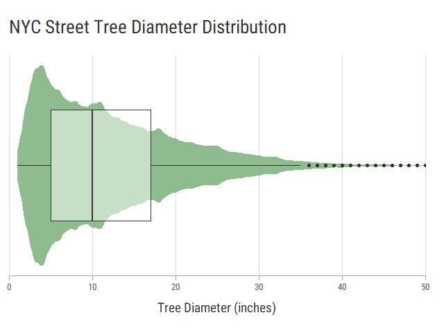 A violin plot overlayed with a box plot.
Any tree over 5 inches in diameter (the first quartile) should be considered old enough to include. Let’s map the oldest trees in NYC.
-- SQL
-- get all the trees from 2015 that match records from 1995
-- if the genuses match and
-- if the diameter > 5 inches and
-- the tree is alive
SELECT trees2015.tree_dbh,
       trees2015.status,
       lower(trees2015.spc_common) AS species_common,
       trees2015.health,
       trees2015.zipcode,
       trees2015.zip_city,
       trees2015.latitude,
       trees2015.longitude,
       CASE instr(trim(trees2015.spc_latin), " ")
        WHEN 0 THEN lower(trim(trees2015.spc_latin) )
        ELSE lower(substr(trees2015.spc_latin, instr(trim(trees2015.spc_latin), " "), -100) )
        END genus2015,
       CASE instr(trim(trees1995.spc_latin), " ")
        WHEN 0 THEN lower(trim(trees1995.spc_latin) )
        ELSE lower(substr(trees1995.spc_latin, instr(trim(trees1995.spc_latin), " "), -100) )
        END genus1995
FROM new_york_tree_census_2015 AS trees2015
     JOIN
     new_york_tree_census_1995 AS trees1995 ON trees2015.tree_id = trees1995.recordid
WHERE genus2015 = genus1995 AND
      trees2015.tree_dbh > 5 AND
      trees2015.status = "Alive";
# R
# the SQL query above is stored in variable q as a string
oldTrees <- dbGetQuery(treeCensus, q)
# disconnect from the database since it's no longer needed for this project
dbDisconnect(treeCensus)
head(oldTrees)
# tree_dbh status species_common health zipcode zip_city latitude longitude genus2015 genus1995
# 1 13 Alive silver maple Good 10312 Staten Island 40.55740 -74.17193 acer acer
# 2 7 Alive ginkgo Good 11374 Rego Park 40.72244 -73.86302 ginkgo ginkgo
# 3 17 Alive london planetree Good 11207 Brooklyn 40.65968 -73.88943 platanus platanus
# 4 16 Alive pin oak Good 11001 Floral Park 40.73641 -73.70546 quercus quercus
# 5 29 Alive london planetree Good 10022 New York 40.75725 -73.96023 platanus platanus
# 6 10 Alive sycamore maple Fair 11358 Flushing 40.75578 -73.80656 acer acer
# get bounding box of the trees
# limit the sample size to 1000 out of 36k
lon <- sample(oldTrees$longitude, size=1000)
lat <- sample(oldTrees$latitude, size=1000)
oldTreeBB <- make_bbox(lon, lat)
# use stamenmap here because it allows a bounding box
ggmap(get_stamenmap(bbox=oldTreeBB,
maptype="toner-background"),
darken=c(0.8, "white")) +
geom_point(data=oldTrees,
mapping=aes(x=longitude, y=latitude),
stroke=0,
alpha=0.1,
color="palegreen4") +
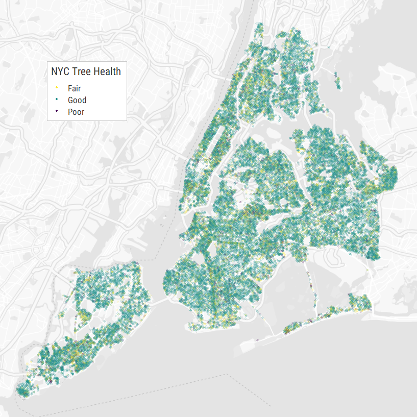
theme_void()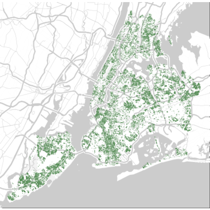 Oldest street trees in New York City in 2015.
Zip Code with the Most Old Trees
The map above is pretty dense, so let’s zoom to the zip code with the most old trees. Start by finding the counts of each zip code in our “oldTrees” dataset.
# R
# get the unique zip codes
uniqueZips <- unique(oldTrees$zipcode)
# convert zip codes to factors so they are considered as categories and not integers
oldTrees$zipcode <- factor(oldTrees$zipcode, levels=uniqueZips)
# create a tibble with unique zip codes and their counts
zipCodes <- tibble(zipcode=uniqueZips, count=tabulate(oldTrees$zipcode))
# sort by count
zipCodes <- arrange(zipCodes, desc(count))
# top 6
head(zipCodes)
# A tibble: 6 × 2
#   zipcode count
#   <int>   <int>
# 1 10312    1862
# 2 10314    1681
# 3 10306    1358
# 4 10309    1143
# 5 11230     679
# 6 11385     673
The top zip code (10312) corresponds to Staten Island, so let’s map it.
# R
# filter table by zip code
oldestZip <- oldTrees[oldTrees$zipcode==10312,]
# get bounding box of the trees
lon <- oldestZip$longitude
lat <- oldestZip$latitude
oldestZipBB <- make_bbox(lon, lat)
# find the center of the bounding box
(oldestZipCenter <- c((oldestZipBB['left'] + oldestZipBB['right'])/2,
(oldestZipBB['top'] + oldestZipBB['bottom'])/2))
# filter table by zip code, exclusive
otherZips <- oldTrees[oldTrees$zipcode!=10312,]
# map the result
# use google maps because it allows larger scales
ggmap(get_googlemap(center=oldestZipCenter,
maptype="roadmap",
zoom=13,
color="bw",
style="feature:all|element:labels|visibility:off"),
darken=c(0.6, "white")) +
geom_point(data=otherZips,
mapping=aes(x=longitude, y=latitude),
stroke=0,
alpha=0.3,
color="dodgerblue4") +
geom_point(data=oldestZip,
mapping=aes(x=longitude, y=latitude),
stroke=0,
alpha=0.5,
color="palegreen4") +
theme_void()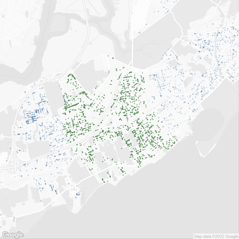 Oldest street trees in Staten Island, NY 10312 in 2015.
Themes
I created two custom themes for the plots in this post. I omitted them above for brevity.
# R
# define the font to use
windowsFonts(RobotoCond = windowsFont("Roboto Condensed"))

# define styles for reuse
titleMargin <- margin(t=10,r=10,b=20,l=10)
gridColor <- "#DDDDDD"
axisColor <- "#AAAAAA"
lineColor <- "#666666"

# define a theme for vertical plots
verticalTheme <- theme(text=element_text(family = "RobotoCond",
                                       color="#333333"),
                     title=element_text(size=14),
                     plot.title=element_text(margin=titleMargin,
                                            size=20),
                     axis.title.y=element_text(margin=titleMargin),
                     axis.title.x=element_text(margin=titleMargin),
                     axis.text=element_text(size=10),
                     axis.ticks.y=element_blank(),
                     axis.ticks.x=element_line(color=axisColor),
                     axis.ticks.length=unit(5, units="pt"),
                     axis.line.x=element_line(color=axisColor),
                     legend.text=element_text(size=12),
                     plot.background=element_blank(),
                     plot.margin=margin(10,20,0,5),
                     panel.background=element_blank(),
                     panel.grid.major=element_blank(),
                     panel.grid.minor=element_blank(),
                     panel.grid.major.y=element_line(color=gridColor))

# define a theme for horizontal density plots
densityTheme <- theme(text=element_text(family = "RobotoCond",
                                         color="#333333"),
                       title=element_text(size=14),
                       plot.title=element_text(margin=titleMargin,
                                            size=20),
                       axis.title.y=element_blank(),
                       axis.title.x=element_text(margin=titleMargin),
                       axis.text.y=element_blank(),
                       axis.text.x=element_text(size=10),
                       axis.ticks.y=element_blank(),
                       axis.ticks.x=element_line(color=axisColor),
                       axis.ticks.length=unit(5, units="pt"),
                       axis.line.x=element_line(color=axisColor),
                       legend.text=element_text(size=12),
                       plot.background=element_blank(),
                       plot.margin=margin(10,20,0,5),
                       panel.background=element_blank(),
                       panel.grid.major=element_blank(),
                       panel.grid.minor=element_blank(),
                       panel.grid.major.x=element_line(color=gridColor))
This entire script is hosted on Github.